Course Material [2]
5. Plot and Graphics
Some commonly used functions
plot()points()lines()abline()
x<- 1:5
y<- c(3, 2, 4, 1, 5)
plot(x, y, type = "p", main = "point")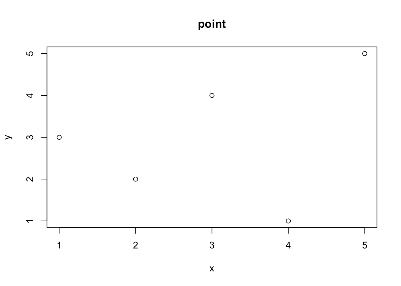
plot(y, type = "p", main = "point")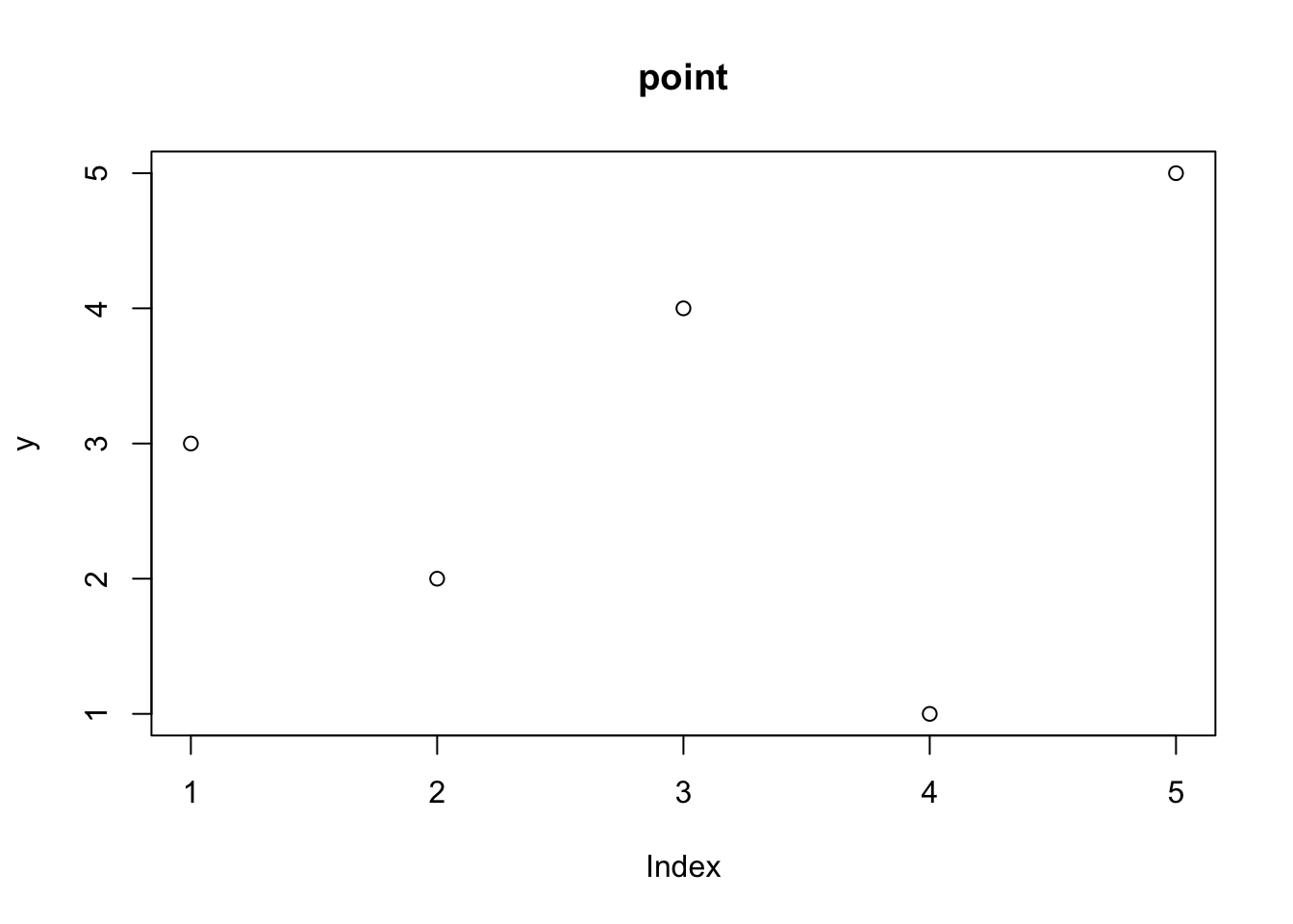
plot(x, y, type = "l", main = "line")
plot(x, y, type = "o", main = "line and point")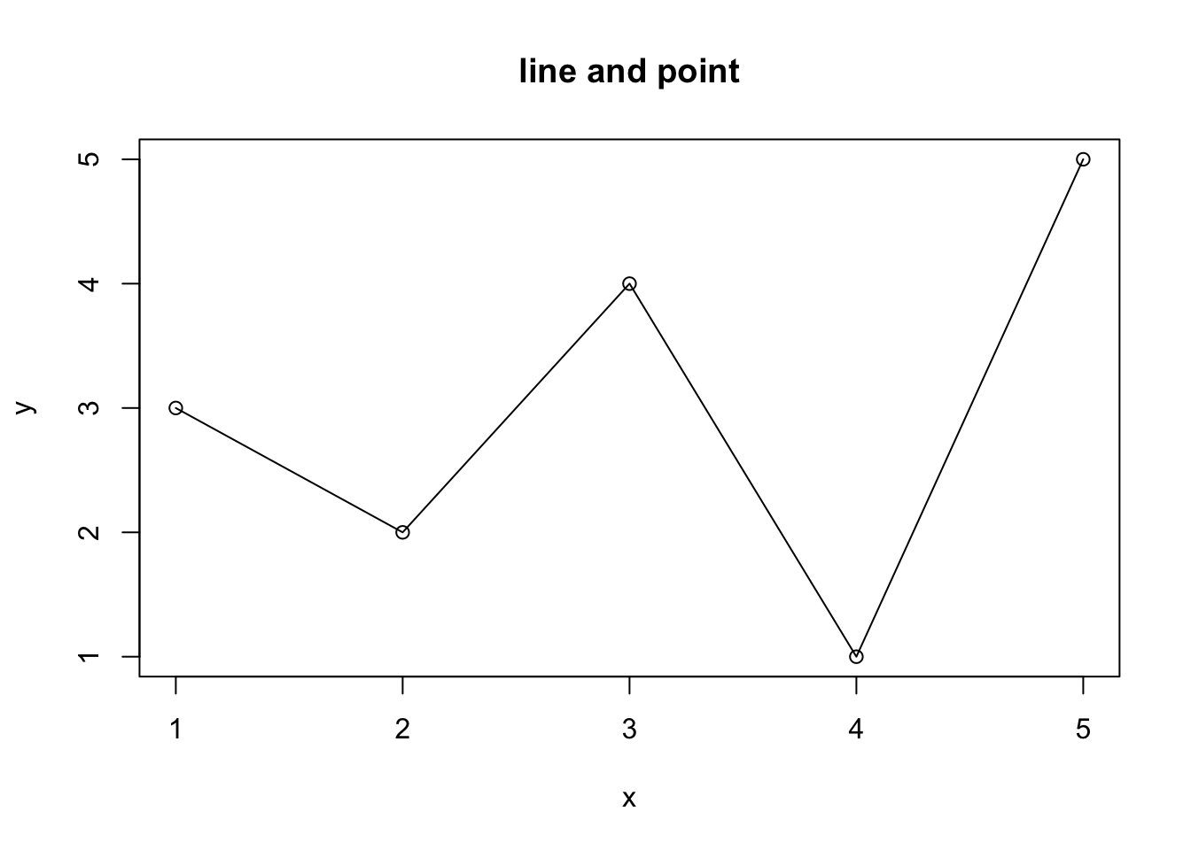
Change the label, scale of axes
x<- 1:5
y<- c(3, 2, 4, 1, 5)
plot(x, y, type = "p", xlab = "x values", ylab = "y values")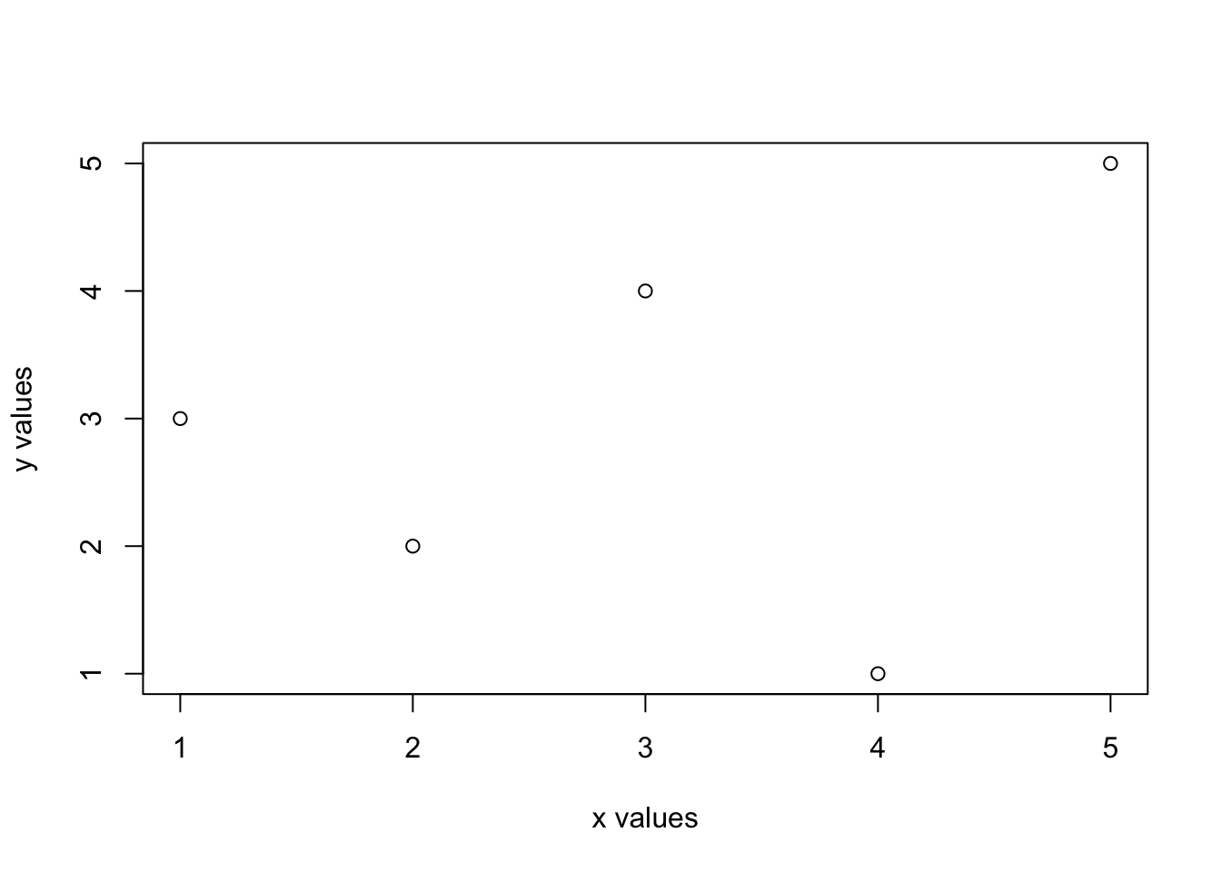
plot(x, y, type = "p", xlim = c(0, 6), ylim = c(-1, 7))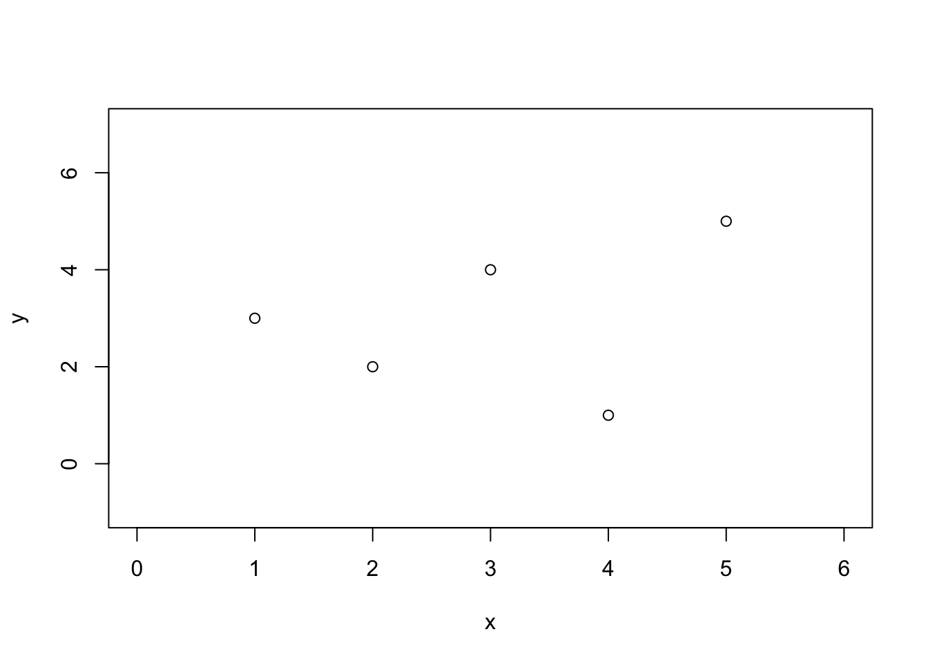
Add points, lines, and legend
x<- seq(0, 2*pi, .2)
plot(x, sin(x), type = "o", pch = 19)
points(x, cos(x), pch = 19, col = 2)
lines(x, cos(x), lty = 2, col = 2)
legend(4, 1, legend = c("sin", "cos"), pch = c(1, 19), lty = c(1, 2), col = c(1, 2))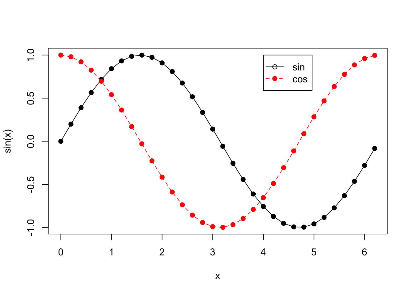
pch: point style
plot(sapply(1:5, function(x) rep(x, 5)), rep(5:1, 5),
     pch = 1:25, xlab = "", ylab = "", main = "", xlim = c(0.7, 5.2), axes = F)

text(sapply(1:5, function(x) rep(x, 5)) -.2, rep(5:1, 5), 1:25)
lty: line style
plot(NULL, xlim = c(0,4), ylim = c(1,6), xlab = "", ylab = "", axes = F)
for(i in 1:6){
  y_pos<- 6:1
  lines(c(1, 4), c(y_pos[i], y_pos[i]), lty = i)
  text(0.5, i, paste("lty = ", y_pos[i]))
}
color: color
plot(sapply(1:5, function(x) rep(x, 5)), rep(5:1, 5),
     pch = 16, col = 1:25, xlab = "", ylab = "", main = "", xlim = c(0.7, 5.2), axes = F)

text(sapply(1:5, function(x) rep(x, 5)) -.2, rep(5:1, 5), 1:25)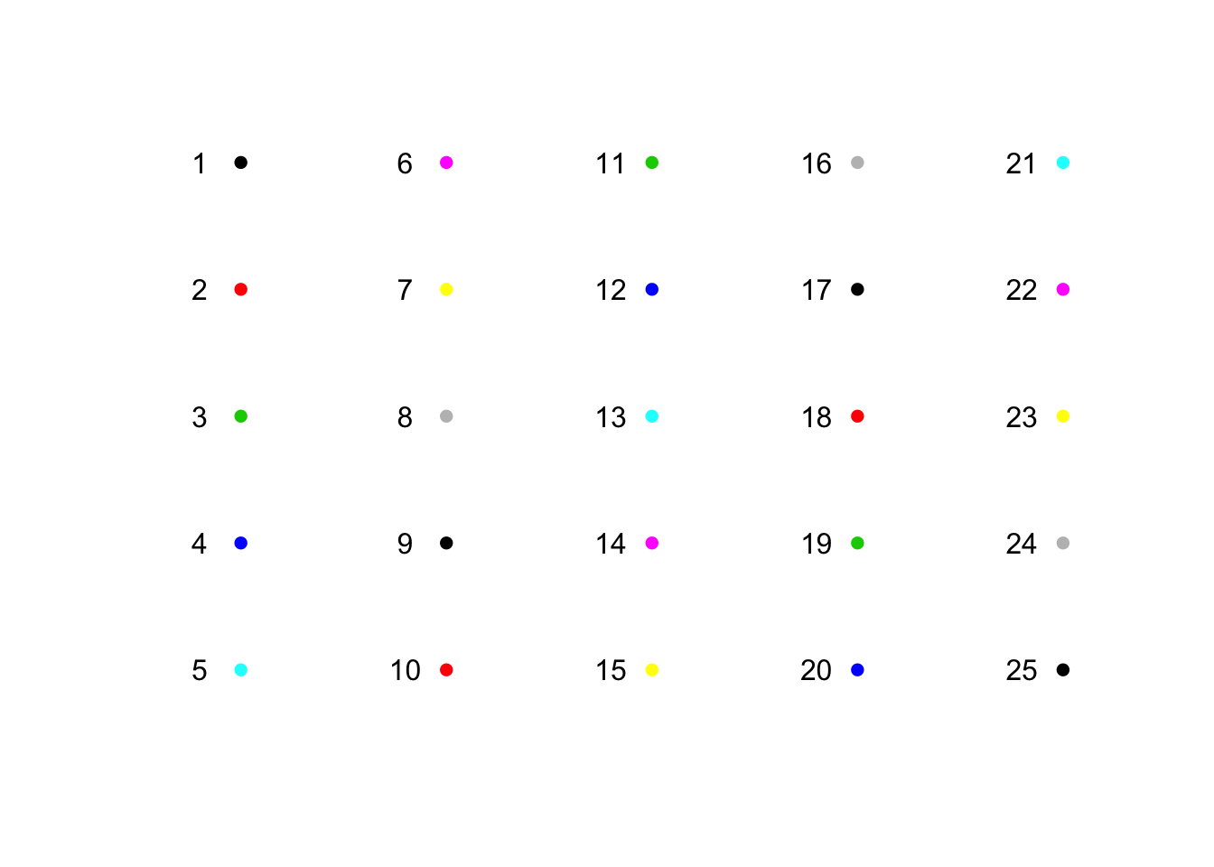
Histogram
attach(iris)
hist(Sepal.Length)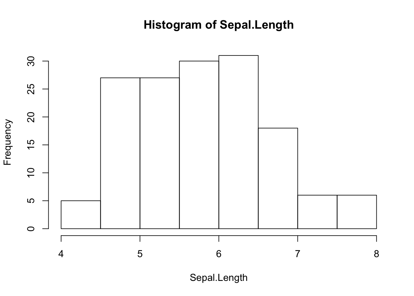
Barplot
attach(chickwts)
barplot(table(feed))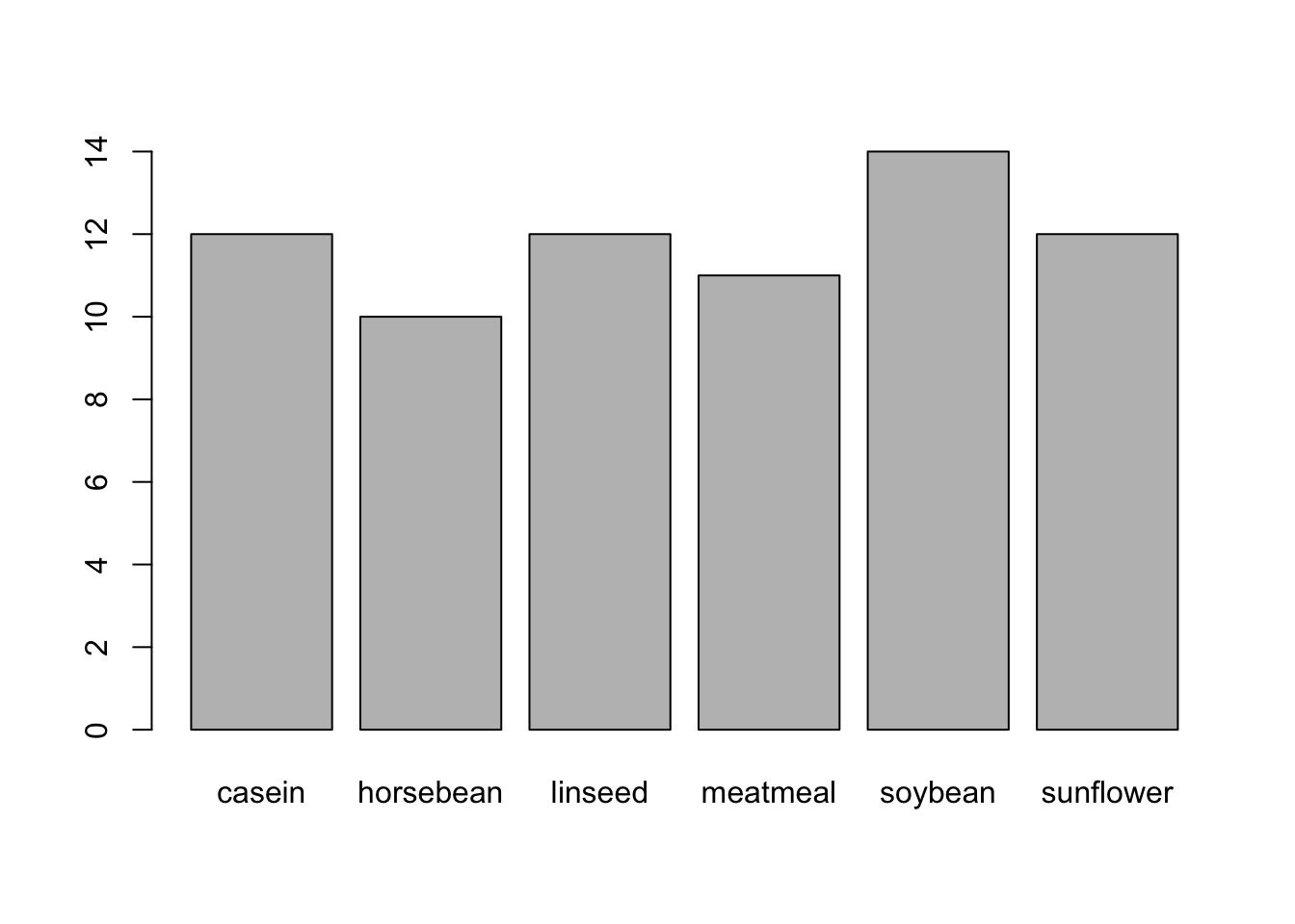
Boxplot
boxplot(weight)
Group-wise boxplot
boxplot(weight~feed)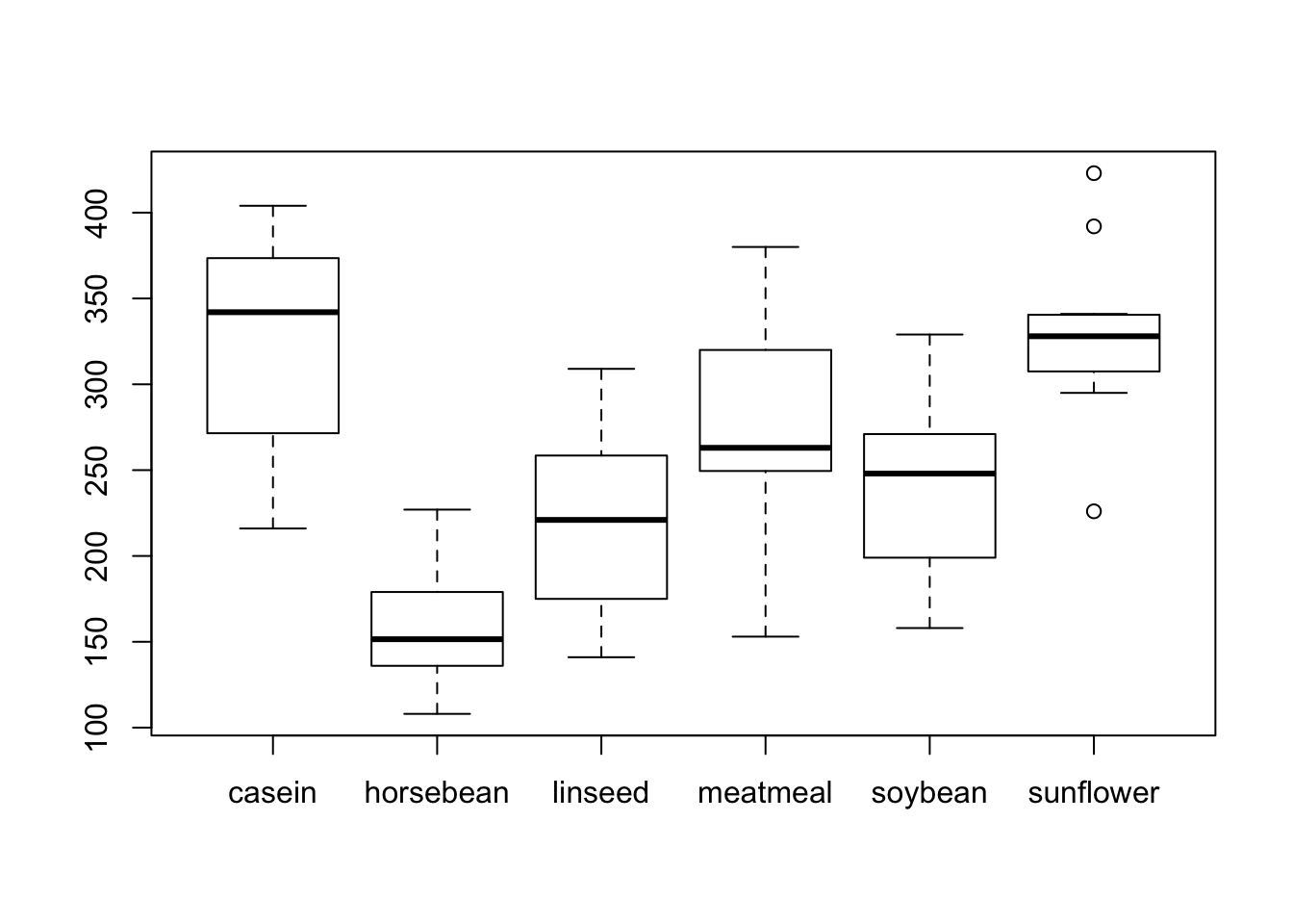
Multiple plots
par(mfrow = c(2,2))
barplot(table(feed))
hist(weight)
boxplot(weight)
boxplot(weight~feed)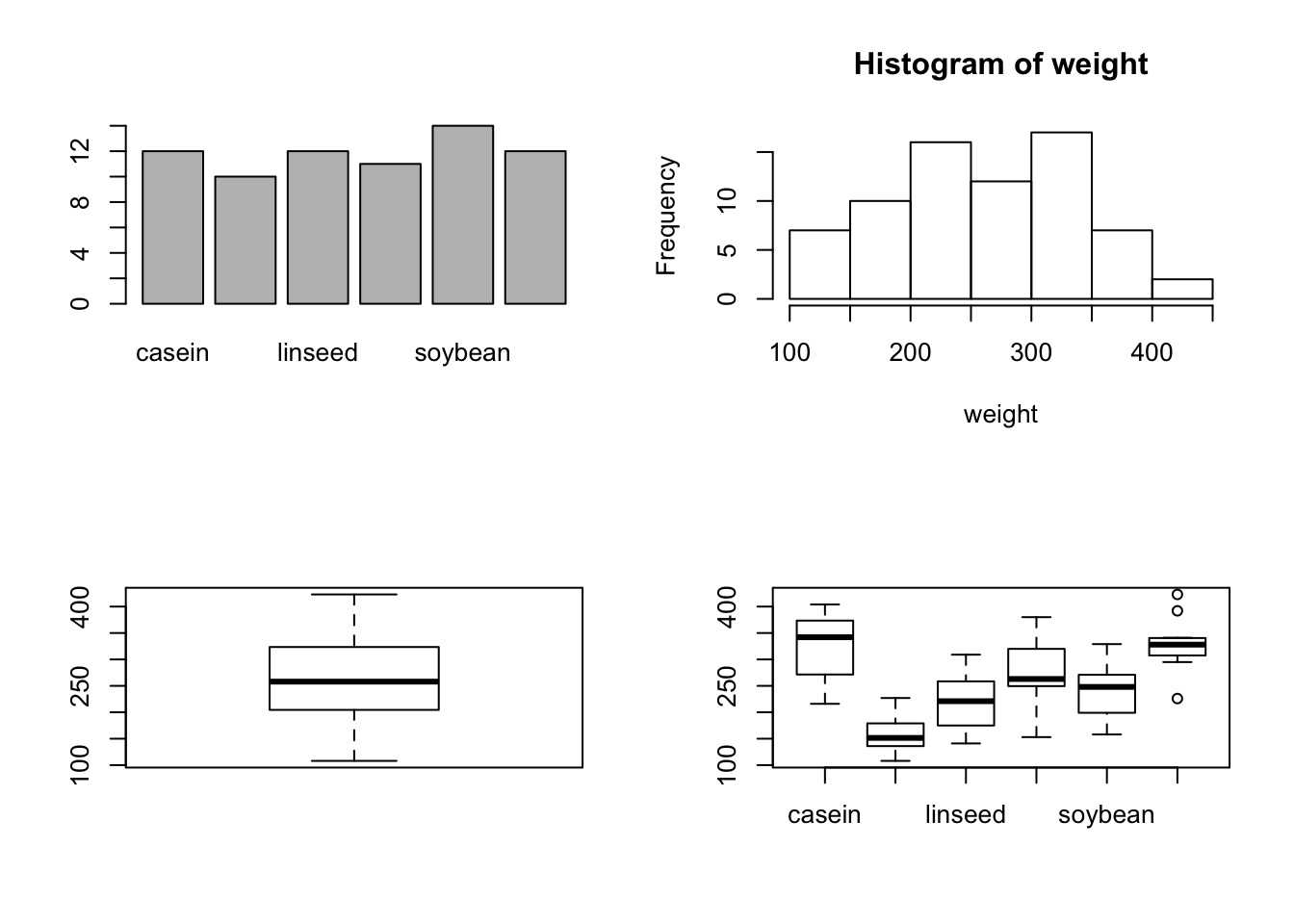
attach(chickwts)
#> The following objects are masked from chickwts (pos = 3):
#>
#>     feed, weight
layout(matrix(c(1,1,2,3), 2, 2, byrow = TRUE))
boxplot(weight~feed)
hist(weight)
boxplot(weight)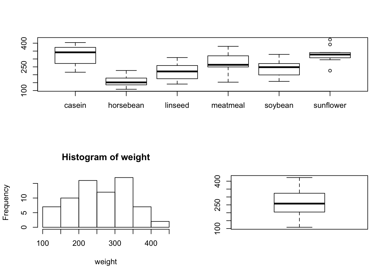
Scatter plot for more than 2 variables
pairs(trees)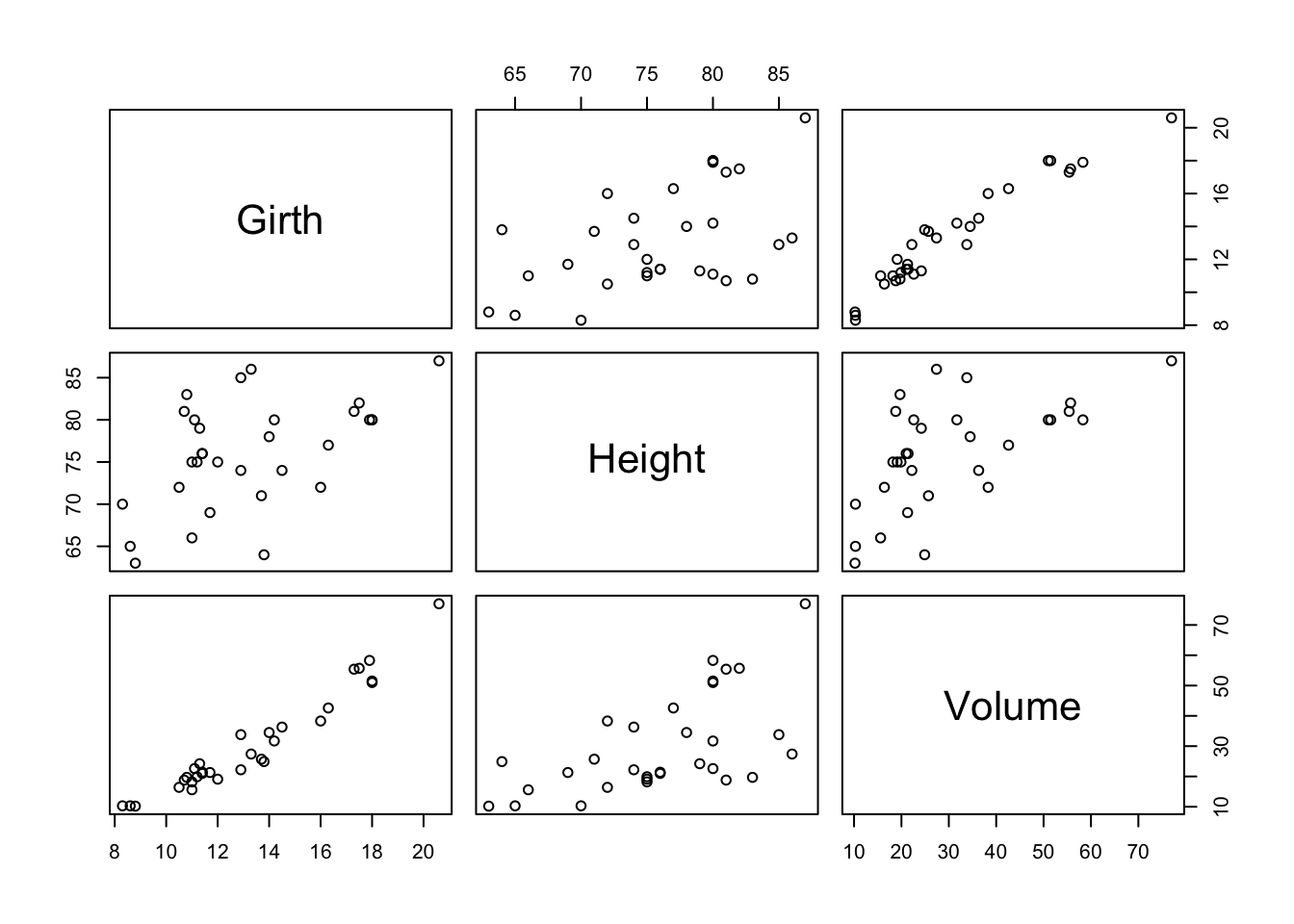
Plot into a file
png(file = "exmple.png", bg = "transparent")
plot(x, sin(x), type = "o")
dev.off()
Exercise 5
(attach the corresponding plots to the email)
Use the dataset
airquality. Draw a scattar to show the relationship between variablesOzoneandSolar.R. Show the points withWindvalues greater than 9.7 in red, otherwise in black.[!!! Only for practice (answers proviede below)] Make plot to monitor the convergence of the exponential function (\(e^x \ = \sum_{n=0}^{\infty} \frac{x^{n}}{n!}\)) with \(x = 5\).
taylor_appox<- function(x){
  function(N){
    sum(
     sapply(0:N, function(n) x^n / factorial(n))
    )
  }
}

x<- 5
taylor_appox_N<- taylor_appox(x)

N_vec<- 1:20
approx_val<- sapply(N_vec, function(N){
  taylor_appox_N(N)
})
plot(N_vec, approx_val)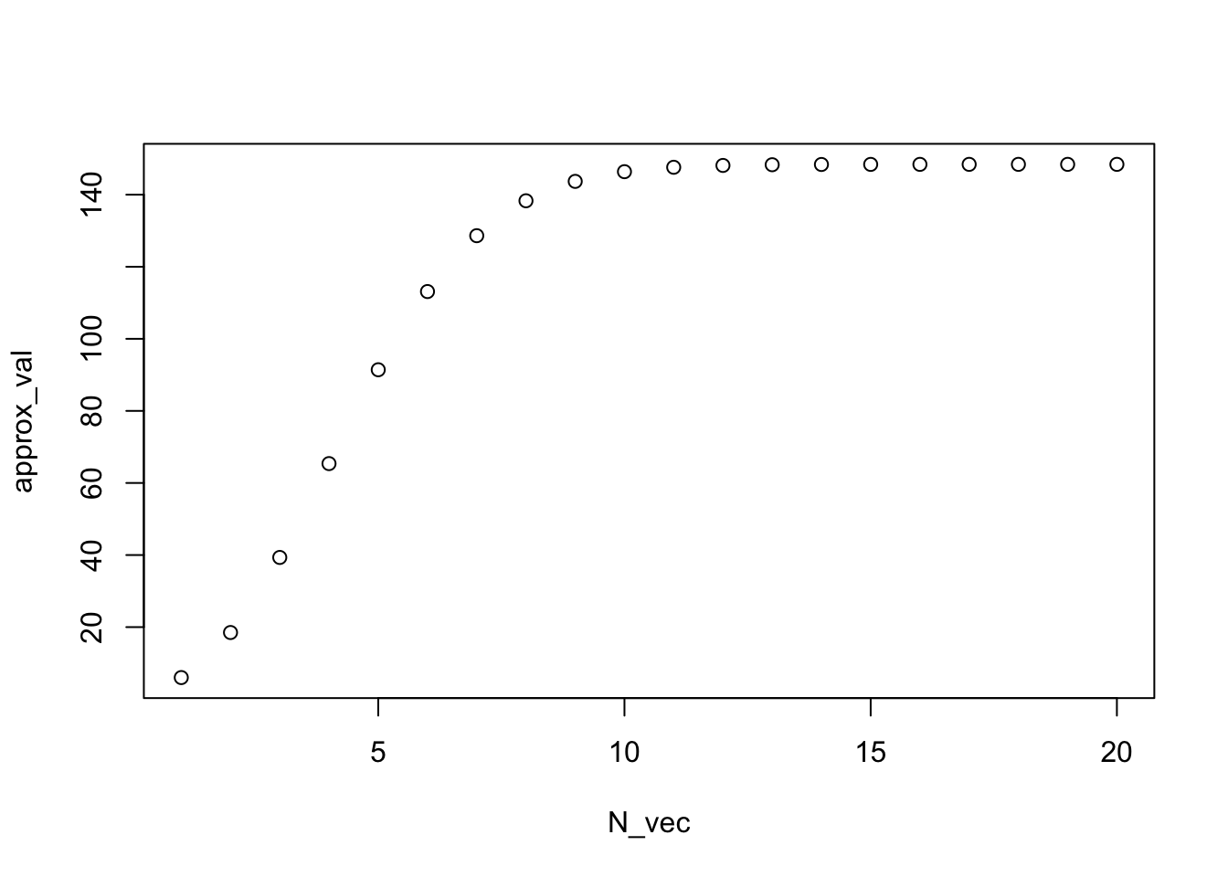
Use the dataset
sleep. Put a histogram and a boxplot in one plot to show the overall pattern of the increased sleeping time (variableextra).Use the dataset
sleep. Use boxplots to show the difference of the increased sleeping time between two groups.Use the vector
islands. Use barplots to disply the area of the 2 smallest islands and the 2 biggest islands. (Hint. you can usesort(, decreasing = )to sort a vector.)Use dataset
iris. Make a scatter plot of four variablesSepal.Length,Sepal.Width,Petal.LengthandPetal.Width. Show different species in different colors. (e.g.setosain black,versicolorin red andvirginicain green)Use dataset
ChickWeight. From each of theDietgroup, select 1 chick (identifier variableChick). Make a time series plot to show the weight changing over time of the 4 selected chicks, each in one different color. Put a legend on the plot which contains the information of the selected chicks (DietandChick) and their corresponding colors.
6. Statistical Computation
Descriptive Statistics
mean(): meanvar(): variancesd(): standard deviationmedian(): medianquantile(): sample quantilesmin(): minimummax(): maximumrange(): range (minimum and maximum values)summary(): summaryIQR(): interquartile rangecov(): covariancecor(): correlation
quantile(trees$Height, prob = c(.05, .15, .25, .75))
#>   5%  15%  25%  75%
#> 64.5 69.5 72.0 80.0

mean(trees$Height)
#> [1] 76

var(trees$Height)
#> [1] 40.6

cov(trees)
#>            Girth   Height    Volume
#> Girth   9.847914 10.38333  49.88812
#> Height 10.383333 40.60000  62.66000
#> Volume 49.888118 62.66000 270.20280

cor(trees)
#>            Girth    Height    Volume
#> Girth  1.0000000 0.5192801 0.9671194
#> Height 0.5192801 1.0000000 0.5982497
#> Volume 0.9671194 0.5982497 1.0000000

summary(trees)
#>      Girth           Height       Volume
#>  Min.   : 8.30   Min.   :63   Min.   :10.20
#>  1st Qu.:11.05   1st Qu.:72   1st Qu.:19.40
#>  Median :12.90   Median :76   Median :24.20
#>  Mean   :13.25   Mean   :76   Mean   :30.17
#>  3rd Qu.:15.25   3rd Qu.:80   3rd Qu.:37.30
#>  Max.   :20.60   Max.   :87   Max.   :77.00

apply(trees, 2, range)
#>      Girth Height Volume
#> [1,]   8.3     63   10.2
#> [2,]  20.6     87   77.0

apply(trees, 2, sd)
#>     Girth    Height    Volume
#>  3.138139  6.371813 16.437846

apply(trees, 2, IQR)
#>  Girth Height Volume
#>    4.2    8.0   17.9
Distributions
dxxx: densityqxxx: quantilepxxx: cumulativerxxx: random samples
E.g. Normal distribution
dnorm(0, 0, 1)
#> [1] 0.3989423
qnorm(.975, 0, 1)
#> [1] 1.959964
pnorm(1.96, 0, 1)
#> [1] 0.9750021
rnorm(10, 0, 1)
#>  [1]  0.4553153  0.7204558 -0.2075951  0.6949459  1.1768098  1.1065208
#>  [7] -1.8412702  0.5858104 -0.1618266  1.8454567

x<- rnorm(100000, 0, 1)
hist(x, freq = F, ylim = c(0, .5))
lines(density(x))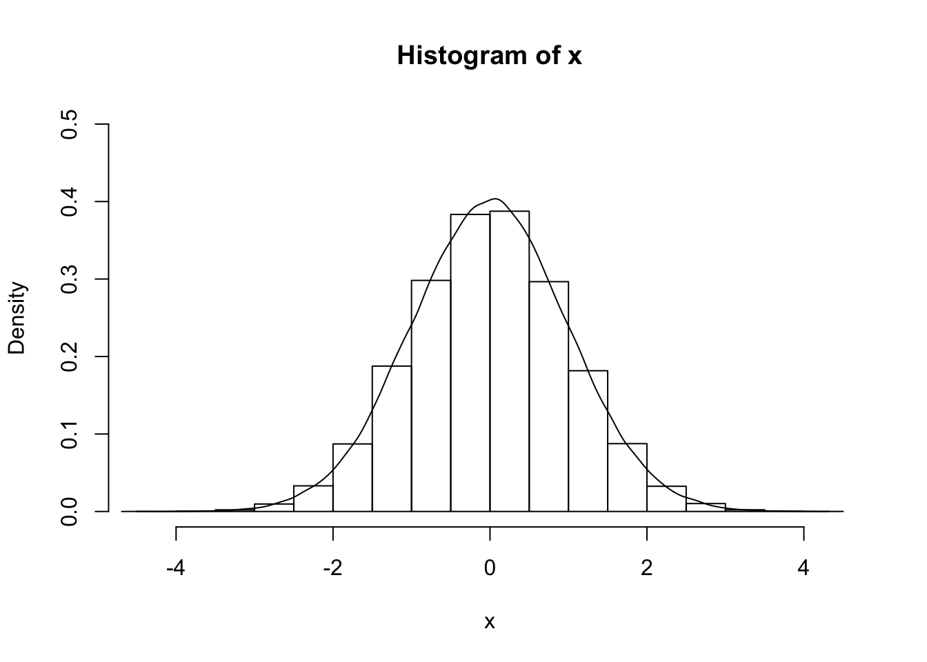
density: kernel density estimation.
E.g. Beta distribution
dbeta(0.5, 1, 2)
#> [1] 1
qbeta(.975, 1, 2)
#> [1] 0.8418861
pbeta(0.5, 1, 2)
#> [1] 0.75
rbeta(10, 1, 2)
#>  [1] 0.12071798 0.60483411 0.04445160 0.17540246 0.53954067 0.02143565
#>  [7] 0.03987329 0.42490878 0.41748311 0.01702245
E.g. Gamma distribution
dgamma(10, 5)
#> [1] 0.01891664
qgamma(.5, 5)
#> [1] 4.670909
pgamma(10, 5)
#> [1] 0.9707473
rgamma(10, 5)
#>  [1]  3.215150  4.609378 11.020029  6.261862  6.540449  2.583292 12.648890
#>  [8]  1.609669  4.426637  8.138750
Other commonly used distributions
- Uniform (
dunif,qunif,punif,runif) - Binomial (
dbinom,qbinom,pbinom,rbinom) - Poisson (
dpois,qpois,ppois,rpois) - Cauchy (
dcauchy,qcauchy,pcauchy,rcauchy) - Student t (
dt,qt,pt,rt) - Weibull (
dweibul,qweibul,pweibul,rweibul) - Geometric (
dgeom,qgeom,pgeom,rgeom) - …
Student’s t-test
attach(iris)
#> The following objects are masked from iris (pos = 5):
#>
#>     Petal.Length, Petal.Width, Sepal.Length, Sepal.Width, Species
levels(Species)
#> [1] "setosa"     "versicolor" "virginica"
t.test(Sepal.Length[Species == "setosa"], Sepal.Length[Species == "versicolor"])
#>
#>  Welch Two Sample t-test
#>
#> data:  Sepal.Length[Species == "setosa"] and Sepal.Length[Species == "versicolor"]
#> t = -10.521, df = 86.538, p-value < 2.2e-16
#> alternative hypothesis: true difference in means is not equal to 0
#> 95 percent confidence interval:
#>  -1.1057074 -0.7542926
#> sample estimates:
#> mean of x mean of y
#>     5.006     5.936
Analysis of Variance (ANOVA)
aov_res<- aov(Sepal.Length ~ Species)
summary(aov_res)
#>              Df Sum Sq Mean Sq F value Pr(>F)
#> Species       2  63.21  31.606   119.3 <2e-16 ***
#> Residuals   147  38.96   0.265
#> ---
#> Signif. codes:  0 '***' 0.001 '**' 0.01 '*' 0.05 '.' 0.1 ' ' 1
Linear Regression
attach(airquality)
lm_res<- lm(Ozone ~ Solar.R + Wind + Temp)
summary(lm_res)
#>
#> Call:
#> lm(formula = Ozone ~ Solar.R + Wind + Temp)
#>
#> Residuals:
#>     Min      1Q  Median      3Q     Max
#> -40.485 -14.219  -3.551  10.097  95.619
#>
#> Coefficients:
#>              Estimate Std. Error t value Pr(>|t|)
#> (Intercept) -64.34208   23.05472  -2.791  0.00623 **
#> Solar.R       0.05982    0.02319   2.580  0.01124 *
#> Wind         -3.33359    0.65441  -5.094 1.52e-06 ***
#> Temp          1.65209    0.25353   6.516 2.42e-09 ***
#> ---
#> Signif. codes:  0 '***' 0.001 '**' 0.01 '*' 0.05 '.' 0.1 ' ' 1
#>
#> Residual standard error: 21.18 on 107 degrees of freedom
#>   (42 observations deleted due to missingness)
#> Multiple R-squared:  0.6059, Adjusted R-squared:  0.5948
#> F-statistic: 54.83 on 3 and 107 DF,  p-value: < 2.2e-16
Model selction via stepwise approach
lm_step<- step(lm_res)
#> Start:  AIC=681.71
#> Ozone ~ Solar.R + Wind + Temp
#>
#>           Df Sum of Sq   RSS    AIC
#> <none>                 48003 681.71
#> - Solar.R  1    2986.2 50989 686.41
#> - Wind     1   11641.6 59644 703.82
#> - Temp     1   19049.9 67053 716.81
summary(lm_step)
#>
#> Call:
#> lm(formula = Ozone ~ Solar.R + Wind + Temp)
#>
#> Residuals:
#>     Min      1Q  Median      3Q     Max
#> -40.485 -14.219  -3.551  10.097  95.619
#>
#> Coefficients:
#>              Estimate Std. Error t value Pr(>|t|)
#> (Intercept) -64.34208   23.05472  -2.791  0.00623 **
#> Solar.R       0.05982    0.02319   2.580  0.01124 *
#> Wind         -3.33359    0.65441  -5.094 1.52e-06 ***
#> Temp          1.65209    0.25353   6.516 2.42e-09 ***
#> ---
#> Signif. codes:  0 '***' 0.001 '**' 0.01 '*' 0.05 '.' 0.1 ' ' 1
#>
#> Residual standard error: 21.18 on 107 degrees of freedom
#>   (42 observations deleted due to missingness)
#> Multiple R-squared:  0.6059, Adjusted R-squared:  0.5948
#> F-statistic: 54.83 on 3 and 107 DF,  p-value: < 2.2e-16
Prediction
input<- data.frame("Solar.R" = c(10, 100), "Wind" = c(20, 5), "Temp" = c(76, 76))
predict(lm_step, input)
#>         1         2
#> -4.856638 50.531085
Exercise 6
Use the dataset
iris, calculate the corrlations among variablesSepal.Length,Sepal.Width,Petal.LengthandPetal.Width.Use the dataset
iris, calculate the summary statistics of variablesSepal.Length,Sepal.Width,Petal.LengthandPetal.Width.Exploring Centrial Limit Theorem. Generate 100 samples from a poisson distribution (
rpois) with parameter \(\lambda = 2\), calculate the mean value out of the 100 samples. Repeate the process 10000 times. Make a histogram of the 10000 mean values. Check the empirical mean and the standard deviation of the 10000 mean values, compare to the theoretical values \(\mu = 2\) and \(\sigma = \frac{\sqrt{2}}{10}\).Use the dataset
sleep, conduct a statistical test of the hypothesis that there is no difference of the increased slepping hours between two groups. The significant level \(\alpha = 0.05\). (Hint:paired = T).Use the dataset
chickwts, conduct a statistical test of the hypothesis that the feed type doesn’t affect the weight of chicks.Use the dataset
cars, build a linear model to examine how the speed (speed) affacts the stopping distance (dist).
7. Packages
The packages such as stats, base are autimatically loaded.
(.packages())
#> [1] "stats"     "graphics"  "grDevices" "utils"     "datasets"  "methods"
#> [7] "base"
You can use library to load packages which are already installed.
Example: Single-Layer Neurual Network
library(nnet)

## split data into training and testing datasets
n_samples<- nrow(iris)
train_ind<- sample(1:n_samples, n_samples * (4/5))
test_ind<- (1:n_samples)[-train_ind]

train_dat<- iris[train_ind,]
test_dat<- iris[test_ind,]

nn_model<- nnet(Species ~., linout = T, size = 5, data = train_dat)
#> # weights:  43
#> initial  value 172.752842
#> iter  10 value 22.585936
#> iter  20 value 5.743512
#> iter  30 value 4.760731
#> iter  40 value 4.750755
#> iter  50 value 4.749318
#> iter  60 value 4.749295
#> iter  70 value 4.749148
#> iter  80 value 4.745243
#> iter  90 value 4.737078
#> iter 100 value 4.359974
#> final  value 4.359974
#> stopped after 100 iterations

pred_nn<- predict(nn_model, test_dat, type = 'class')

## Accuracy
table(test_dat$Species == pred_nn) / nrow(test_dat)
#>
#>      FALSE       TRUE
#> 0.03333333 0.96666667
Example: Decision Tree
library(rpart)

cart_model<- rpart(Species ~., data = test_dat)

pred_cart<- predict(cart_model, test_dat, type = 'class')

## Accuracy
table(test_dat$Species == pred_cart) / nrow(test_dat)
#>
#>     FALSE      TRUE
#> 0.2666667 0.7333333
Use install.packages() to install package.
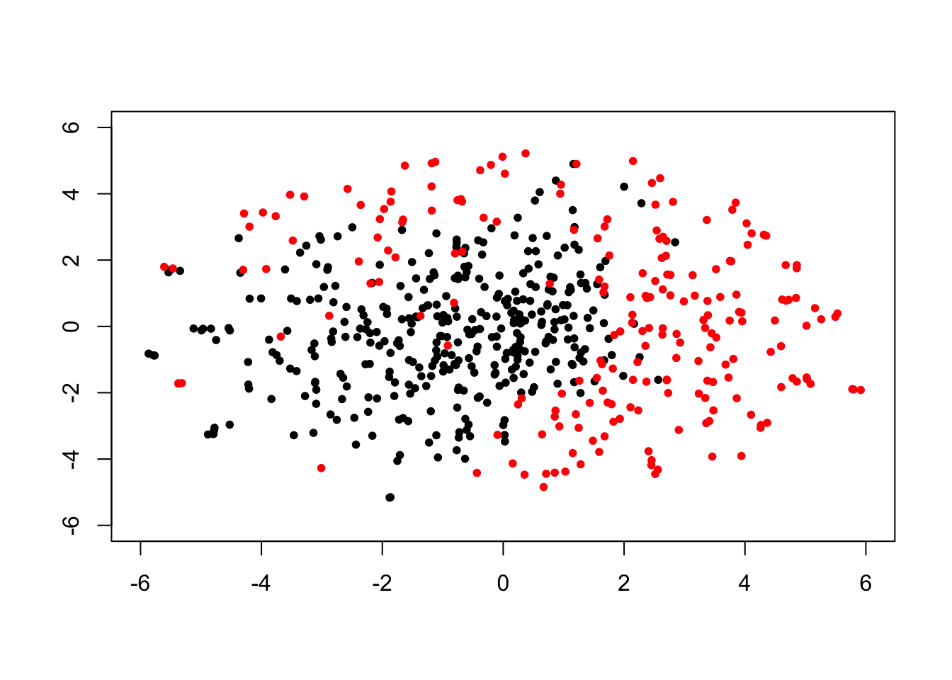
Example: Use t-SNE for dimensionality reduction, visualizing breast cancer data.
library(tsne)

url<- "https://archive.ics.uci.edu/ml/machine-learning-databases/breast-cancer-wisconsin/wdbc.data"
exp_dat<- read.table(url, sep = ",", header = F)

tsne_res<- tsne(exp_dat[, 3:32], perplexity = 100)
#> sigma summary: Min. : 0.38658523478823 |1st Qu. : 0.61806546548001 |Median : 0.648107496657062 |Mean : 0.651623332613159 |3rd Qu. : 0.67963590493686 |Max. : 1.05004711205922 |
#> Epoch: Iteration #100 error is: 15.1274103570016
#> Epoch: Iteration #200 error is: 1.03644698502553
#> Epoch: Iteration #300 error is: 1.01957670964693
#> Epoch: Iteration #400 error is: 1.01153505500181
#> Epoch: Iteration #500 error is: 1.01149416125303
#> Epoch: Iteration #600 error is: 1.01149414953472
#> Epoch: Iteration #700 error is: 1.01149414953464
#> Epoch: Iteration #800 error is: 1.01149414953464
#> Epoch: Iteration #900 error is: 1.01149414953464
#> Epoch: Iteration #1000 error is: 1.01149414953464

plot(tsne_res[which(exp_dat$V2 == "B"), ], col = 1, pch = 20, xlim = c(-6, 6), ylim = c(-6, 6), xlab = "", ylab = "")
points(tsne_res[which(exp_dat$V2 == "M"), ], col = 2, pch = 20)