Course Material [1]
0. Getting Started!
Why Learn R?
- Free (impotrant)
- Massive statistical packages
- More and more popular in both academia and industry
- … Millions of other reasons
How to access
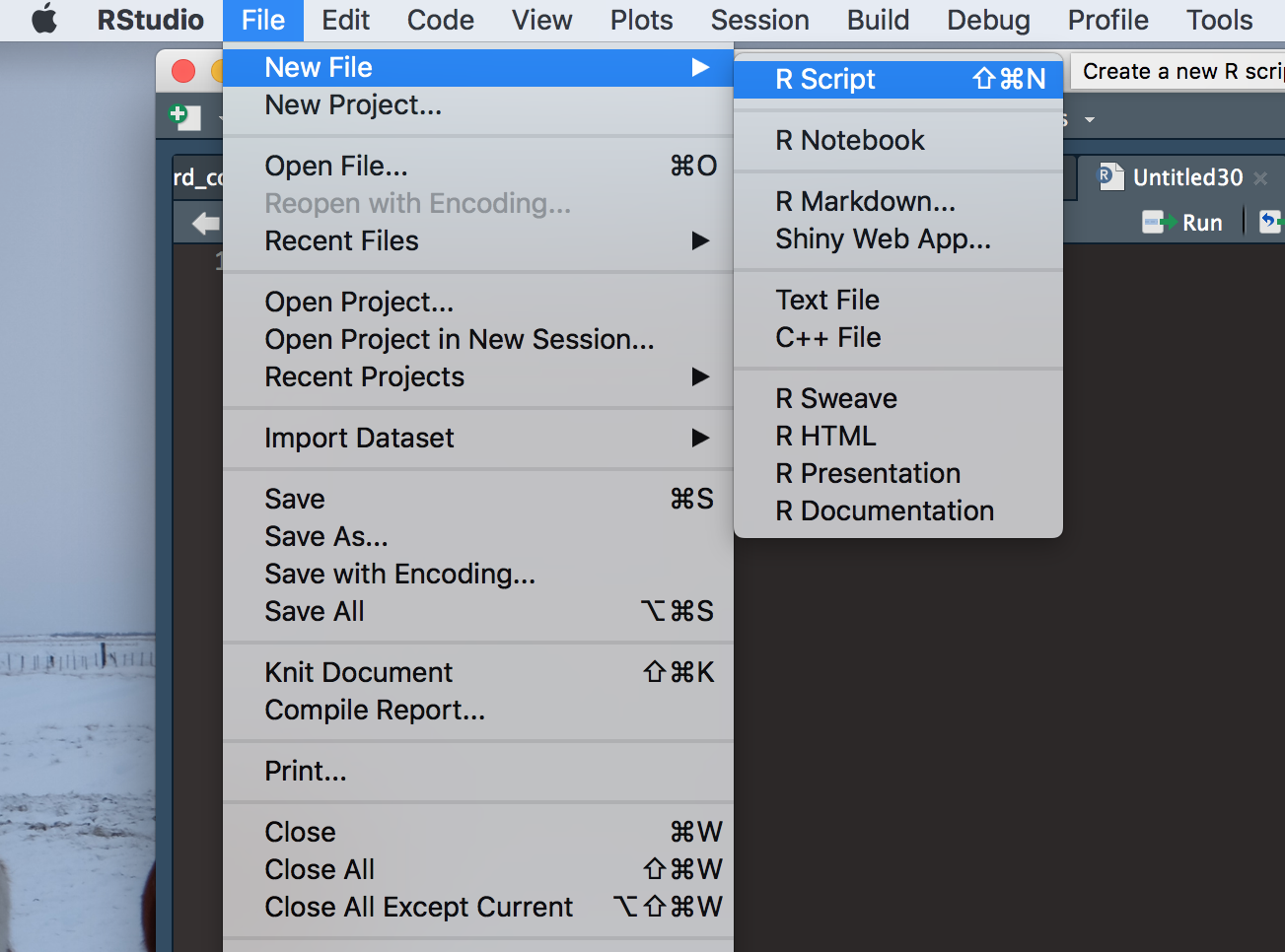
RStudio
Create a script by clicking File >> New File >> R Script
To execute your code, highlight the code you wish to execute and press Ctrl + Enter
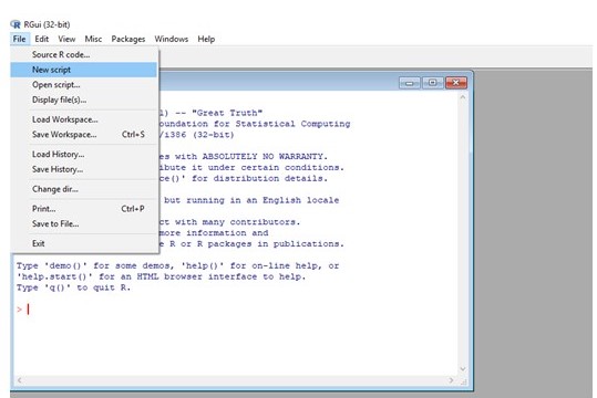
RGui (Windows)
Create a script by clicking File >> New Script
To execute your code, highlight the code you wish to execute and press F5
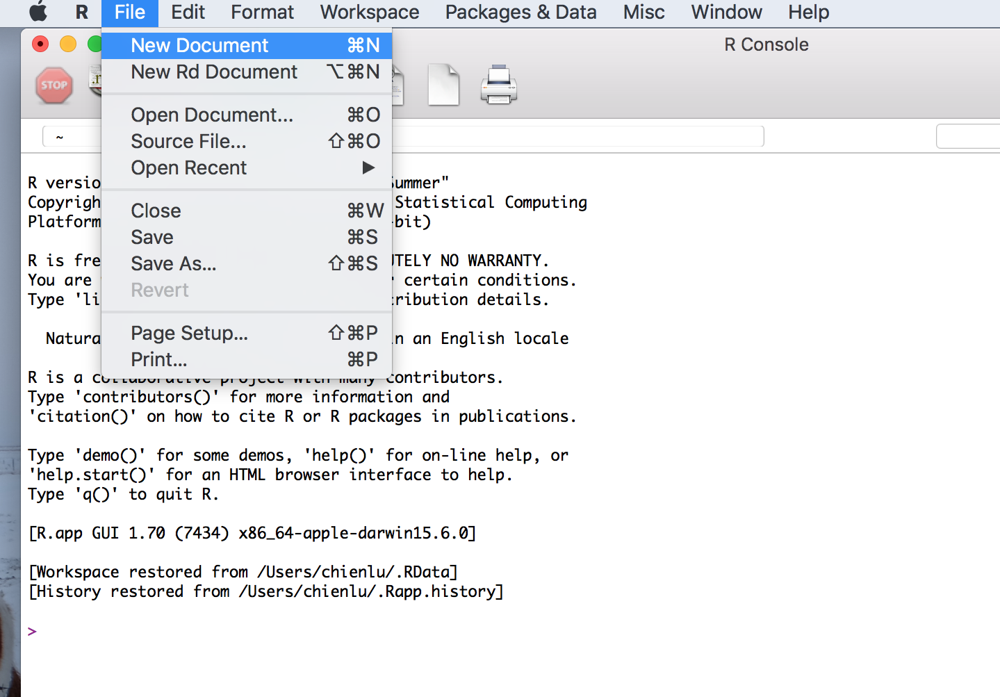
RGui (Mac OS)
Create a script by clicking File >> New Document
To execute your code, highlight the code you wish to execute and press Ctrl + Enter
Set up the working directory
getwd()List all the files/folders under the current working directory
dir()Change the working directory (mind the /)
setwd("/Users/chienlu/Desktop")Quit the R session
q()Some Useful tips
- You can use
#to add comment, the code after will not be executed.
a<- c(1, 2, 3) #I have no idea why I created this vector- Use
?to call R help when you have difficulties.
?dir- When encountering problems, always Google!
Exercise Pack 0
- Check your current directory with the function
getwd. - Change your working directory to your desktop and list all the file/folders
1. R as Calculator
You can start with playing around with R, use it as a calculator
1 + 3
#> [1] 4
6*(5-1)
#> [1] 24
Some useful operators:
+: addition-: subtraction*: multiplication/: divisionx %% y: modulus (Remainder from division)x %/% y: integer division^ or **: exponentiation, e.g.3^2or3**2to compute \(3^2\)
? What is the output of the following code?
-1^2= ?(-1)^2= ?
You can also try out some more complicated (fancier) computations, such as Trigonometric functions (high school nightmare):
sin(): sinecos(): cosinetan(): tangentexp(): Exponential with base elog(): Logarithmlog10(): Logarithm with the base 10sqrt(): Square rootabs(): Absolute valueround(): Round the valuefloor(): Round down the valueceiling(): Round up the valuefactorial(): Factorial functiongamma(): Gamma functiondigamma(): Digamma function- …
? What are the solutions to the following equations
- sin(\(\frac{\pi}{2}\)) = ?
- cos(\(\pi\)) = ?
- tan(\(\frac{\pi}{4}\)) = ?
? Can you verify if the function factorial returns the correct result of \(5!\)?
5*4*3*2*1
#> [1] 120
factorial(5)
#> [1] 120
Exercise Pack 1
- Calculate the volume of a sphere (ball) whose raduis \(r = 2\)
- What is \(35^\circ C\) in Fahrenheit (\(^\circ F\))?
- Use 5 different \(\theta\) values to calculate the result of \(sin(\theta)^2 + cos(\theta)^2\)
- In a right triangle with sides \(a = b = 2 < c\), how long is \(c\)? (Use Pythagorean Theorem)
2. Basic R Objects
Declare value
Use <- to declare a value to an object.
x<- 1
x
#> [1] 1
of course, using = to assign the value also works.
x = 1
x
#> [1] 1
Use class, mode or typeof to check the type of the object.
x<- 1.1
class(x)
#> [1] "numeric"
mode(x)
#> [1] "numeric"
typeof(x)
#> [1] "double"
Working environment
List all the objects under the current working environment.
ls()rm()remove objectobject.size()memory used by the object
Remove all the objects under the current working environment.
rm(list = ls())Numbers
Numeric (real number)
x<- 0.8
class(x)
#> [1] "numeric"
Complex number
x<- 3+0i
class(x)
#> [1] "complex"
Scientific notation
x<- 9.6e-4 Infinity (use is.infinite or is.finite to test)
x<- 1/0
x
#> [1] Inf

is.infinite(x)
#> [1] TRUE
is.finite(x)
#> [1] FALSE
Not a number (undefined result, use is.nan to test)
x<- 0/0
x
#> [1] NaN
is.nan(x)
#> [1] TRUE
Null object (use is.null to test)
x<- NULL
is.null(x)
#> [1] TRUE
Not available/missing value (use is.na to test)
x<- NA
is.na(x)
#> [1] TRUE
is.nan(x)
#> [1] FALSE
Use identical to check if two objects are identical
x<- 1e-3
y<- 0.001
identical(x, y)
#> [1] TRUE
Logical
x<- TRUE
x
#> [1] TRUE

y<- FALSE
y
#> [1] FALSE
or
x<- T
x
#> [1] TRUE

y<- F
y
#> [1] FALSE
Some logical operators
!: not==: exactly equal to!=: not equal to&: and|: or<: less than<=: less than or equal to>: greater than>=: greater than or equal to- ?
!!!T | !F= ? - ?
T > F= ? ?
T + F= ?
Strings
a <- "hello"
a
#> [1] "hello"
class(a)
#> [1] "character"
print("Hello R!")
#> [1] "Hello R!"
Functions
Define your own function with function.
my_square<- function(x){
  x^2
}

my_square(4)
#> [1] 16
or
my_plus<- function(x, y){
  x + y
}

my_plus(2, 3)
#> [1] 5
Note that the last element in the function will be returned as the output value. Or you can use return to specify your output value.
my_square<- function(x){
  return(x^2)
  x^3 # does not affect the output
}

my_square(4)
#> [1] 16
Exercise Pack 2
- Check
identical(as.integer(5), 5.0)andas.integer(5.0) == 5, which one is TRUE? - List all object under the current environment. Check the memory used by the first object in the list.
- Check the types of the following objects (choose one from
class,typeof, andmode)
Inf - InfInf + Inf0/0sin(Inf)Inf/0
- Complete the following function to compute the area of an ellipse where
aandbare the axes.
ellipse_area<- function(a, b){

}

ellipse_area(3, 5)
3. Data structures
Vectors
All the elements in a vector should be of the same object type.
Use c to create a vector
## number
exp_1<- c(1, 2, 3, 4, 5)
exp_1
#> [1] 1 2 3 4 5

## logical
exp_2<- c(TRUE, FALSE, FALSE, TRUE)
exp_2
#> [1]  TRUE FALSE FALSE  TRUE

## string
exp_3<- c("I", "am", "a", "meaningless", "example")
exp_3
#> [1] "I"           "am"          "a"           "meaningless" "example"
or use vector to define an empty vector
emp_vec<- vector()
emp_vec
#> logical(0)
Use seq to create a vector with sequential numbers
a<- seq(from = 1, to = 5, by = 1)
a
#> [1] 1 2 3 4 5
or just simply:
a<- 1:5
a
#> [1] 1 2 3 4 5
Use rep to create a vector with replicate elements
b<- rep(x = 1, times = 3)
b
Use sample to create a vector with random numbers
s<- sample(x = 1:100, size = 5)
s
#> [1] 24 11 63 75 85
Set the seed with set.seed function before sampling if you want to reproduce the result.
sample(1:100, 5)
#> [1] 98 29 45 99 79
sample(1:100, 5)
#> [1] 99 37 66 26 43

set.seed(123)
sample(1:100, 5)
#> [1] 29 79 41 86 91

set.seed(123)
sample(1:100, 5)
#> [1] 29 79 41 86 91min()andmax(): minimum value and maximum value within a vectorwhich.min()andwhich.max(): index of the minimal element and maximal element of a vectorpmin()andpmax(): element-wise minima and maxima of several vectorssum()andprod(): sum and product of the elements of a vectorcumsum()andcumprod(): cumulative sum and product of the elements of a vector
s<- sample(1:100, 5)
s
#> [1]  5 53 88 54 44

min(s)
#> [1] 5
max(s)
#> [1] 88
which.min(s)
#> [1] 1
which.max(s)
#> [1] 3
Concatenate vectors
vec_1<- c(1, 1, 1)
vec_2<- c(2, 2, 2)
vec_join<- c(vec_1, vec_2)
vec_join
#> [1] 1 1 1 2 2 2

vec_3<- c(3, 3, 3)
vec_join<- c(vec_1, vec_2, vec_3)
vec_join
#> [1] 1 1 1 2 2 2 3 3 3
Subset a vector
a<- c(1, 2, 3, 4, 5)

# extract with indices
a[c(1, 3, 5)]
#> [1] 1 3 5

# extract with logicals
a[c(T, F, T, F, T)]
#> [1] 1 3 5

a %% 2 == 1
#> [1]  TRUE FALSE  TRUE FALSE  TRUE

a[(a %% 2 == 1)]
#> [1] 1 3 5

# omit
a[-c(2, 4)]
#> [1] 1 3 5

a[-which(a %% 2 == 0)]
#> [1] 1 3 5
NA values in a vector
a<- c(1, NA, 2, NA, 3)
a
#> [1]  1 NA  2 NA  3

b<- c(1, 2, 3, 4, 5)
b * c(1, NA, 1, NA, 1)
#> [1]  1 NA  3 NA  5

# replace NA with 0
a[is.na(a)]<- 0
a
#> [1] 1 0 2 0 3
Vectorized computation
a<- c(1, 2, 3, 4)
b<- c(5, 6, 7, 8)

a + b
#> [1]  6  8 10 12
a * b
#> [1] 5 12 21 32- ?
a = c(1, 2, 3, 4)andb = c(1, 2, 3)What is the value ofa*b?
Factors
Represente categorical data with specifying levels (e.g. gender, education). A factor is stored as a vector of integers with corresponding labels.
x<- c("Python user", "R user", "C++ user", "R user", "C++ user", "JAVA user", "R user")
f_x<- factor(x)
f_x
#> [1] Python user R user      C++ user    R user      C++ user    JAVA user
#> [7] R user
#> Levels: C++ user JAVA user Python user R user
levels(f_x)
#> [1] "C++ user"    "JAVA user"   "Python user" "R user"
nlevels(f_x)
#> [1] 4
class(f_x)
#> [1] "factor"
summary(f_x)
#>    C++ user   JAVA user Python user      R user
#>           2           1           1           3
or assign the labels you prefer
x<- c(1, 2, 1, 2, 1, 1, 1)
f_x<- factor(x, labels = c("male", "female"))
f_x
#> [1] male   female male   female male   male   male
#> Levels: male female
summary(f_x)
#>   male female
#>      5      2
or by spliting a vector into groups with the function cut
x<- c(12, 64, 47, 36, 31, 64, 25, 34,  6, 89)
f_x<- cut(x, c(0, 14, 64, 100))
f_x
#>  [1] (0,14]   (14,64]  (14,64]  (14,64]  (14,64]  (14,64]  (14,64]
#>  [8] (14,64]  (0,14]   (64,100]
#> Levels: (0,14] (14,64] (64,100]

levels(f_x)<- c("child", "labor", "aged")
summary(f_x)
#> child labor  aged
#>     2     7     1
Matrices
Define a matrix
x<- matrix(1:15, nrow = 3, ncol = 5, byrow = F)
x
#>      [,1] [,2] [,3] [,4] [,5]
#> [1,]    1    4    7   10   13
#> [2,]    2    5    8   11   14
#> [3,]    3    6    9   12   15

x<- matrix(1:15, nrow = 3, ncol = 5, byrow = T)
x
#>      [,1] [,2] [,3] [,4] [,5]
#> [1,]    1    2    3    4    5
#> [2,]    6    7    8    9   10
#> [3,]   11   12   13   14   15
Subset a matrix
x<- matrix(1:15, nrow = 3, ncol = 5)
x[2,]
#> [1]  2  5  8 11 14
x[,1]
#> [1] 1 2 3
x[2,1:3]
#> [1] 2 5 8
x[1:2,c(1,3)]
#>      [,1] [,2]
#> [1,]    1    7
#> [2,]    2    8
Some useful functions and operators for matrix computations:
%*%: matrix multiplication%o%: outer productcrossprod(): cross productt(): tranpose matrixdiag(): diagnaldet(): calculate the determinant of the matrixsolve(): obtain the inverse matrix
A<- matrix(sample(1:10, 4), 2, 2)
B<- matrix(sample(1:10, 6), 2, 3)
A
#>      [,1] [,2]
#> [1,]   10    6
#> [2,]    5    9
B
#>      [,1] [,2] [,3]
#> [1,]    2   10    8
#> [2,]    9    1    5
A%*%B
#>      [,1] [,2] [,3]
#> [1,]   74  106  110
#> [2,]   91   59   85
t(A) %*% A
#>      [,1] [,2]
#> [1,]  125  105
#> [2,]  105  117
crossprod(A)
#>      [,1] [,2]
#> [1,]  125  105
#> [2,]  105  117
solve(A)
#>             [,1]       [,2]
#> [1,]  0.15000000 -0.1000000
#> [2,] -0.08333333  0.1666667
Arrays
Define an array
x<- array(1:24, dim = c(4, 3, 2))
x
#> , , 1
#>
#>      [,1] [,2] [,3]
#> [1,]    1    5    9
#> [2,]    2    6   10
#> [3,]    3    7   11
#> [4,]    4    8   12
#>
#> , , 2
#>
#>      [,1] [,2] [,3]
#> [1,]   13   17   21
#> [2,]   14   18   22
#> [3,]   15   19   23
#> [4,]   16   20   24

x[3,,]
#>      [,1] [,2]
#> [1,]    3   15
#> [2,]    7   19
#> [3,]   11   23
x[3,2,]
#> [1]  7 19
x[3,2,1]
#> [1] 7
Lists
x<- list(name = "miina", age = 25, score = 1, pass = T, gender = "female")
length(x)
#> [1] 5
x$name
#> [1] "miina"
x[2]
#> $age
#> [1] 25
x[[3]]
#> [1] 1
x["pass"]
#> $pass
#> [1] TRUE
x[["gender"]]
#> [1] "female"
Data Frames
A data frame generalized matrix in which each column may have different object types. It can be also seen as aa list of colume vectors with all equal length, thus, the way to extract the colums is the same as how you do on a list.
toy_dat<- data.frame(id = 1:5, age = c(15, 5, 11, 10, 95), city = c("Tampere", "Pori", "Tampere", "Helsinki", "Turku"))
toy_dat
#>   id age     city
#> 1  1  15  Tampere
#> 2  2   5     Pori
#> 3  3  11  Tampere
#> 4  4  10 Helsinki
#> 5  5  95    Turku
toy_dat$id
#> [1] 1 2 3 4 5
toy_dat[2]
#>   age
#> 1  15
#> 2   5
#> 3  11
#> 4  10
#> 5  95
Import and Export Dataset
The example dataset steam_subset.csv can be found here. (Right click -> Save as). The colums are seperated with comma( , ) and the first line is the column names.
Read the data set from a file with read.table, use functions head and str to check the dataset
steam<- read.table(file = "steam_subset.csv", sep = ",", header = T)
head(steam)
#>   UserId Level Showcases Comments Badges
#> 1      1    17         1       24     10
#> 2      2    55         2      105     47
#> 3      3     0         0       11      0
#> 4      4    16         1       15     12
#> 5      5    52         4       98     38
#> 6      6    27         2        5     41
str(steam)
#> 'data.frame':    500 obs. of  5 variables:
#>  $ UserId   : int  1 2 3 4 5 6 7 8 9 10 ...
#>  $ Level    : int  17 55 0 16 52 27 57 14 21 71 ...
#>  $ Showcases: int  1 2 0 1 4 2 5 1 2 7 ...
#>  $ Comments : int  24 105 11 15 98 5 1024 16 25 111 ...
#>  $ Badges   : int  10 47 0 12 38 41 72 10 21 66 ...
or use read.csv to read the file
steam<- read.csv(file = "steam_subset.csv", header = T, sep = ",")
head(steam)
#>   UserId Level Showcases Comments Badges
#> 1      1    17         1       24     10
#> 2      2    55         2      105     47
#> 3      3     0         0       11      0
#> 4      4    16         1       15     12
#> 5      5    52         4       98     38
#> 6      6    27         2        5     41
str(steam)
#> 'data.frame':    500 obs. of  5 variables:
#>  $ UserId   : int  1 2 3 4 5 6 7 8 9 10 ...
#>  $ Level    : int  17 55 0 16 52 27 57 14 21 71 ...
#>  $ Showcases: int  1 2 0 1 4 2 5 1 2 7 ...
#>  $ Comments : int  24 105 11 15 98 5 1024 16 25 111 ...
#>  $ Badges   : int  10 47 0 12 38 41 72 10 21 66 ...
Computation on the variables
mean(steam$Level)
#> [1] 37.648
sd(steam$Level)
#> [1] 68.99508
Attach a dataset
# stick to it
attach(steam)
mean(Level)
#> [1] 37.648
sd(Level)
#> [1] 68.99508

# get rid of it
detach(steam)
Save the dataset to a csv file
write.csv(toy_dat, file = "toy.csv", row.names = F)Exercise Pack 3
- Create a vector
zof length 10 with variance equals to 0 and mean equals to 5. Verify with functionmeanandvar. - Create a function which returns the sum of the maximum and the mininum value of the input vector
- [!!! Only for practice (answers proviede below)] Create a function which approximates the sin function with 4th-order taylor series.
sin_approx<- function(x){
  x - x^3 / factorial(3)
}

sin_approx(0)
#> [1] 0
sin(0)
#> [1] 0

sin_approx(1)
#> [1] 0.8333333
sin(1)
#> [1] 0.841471- Compute the CV (coefficient of variation) values of variables
LevelandBadgesin thesteamdataset. - Create a toy data frame object with at least 5 rows and 3 columns, save it to a .csv file.
4. Computations
Loops
For loop
for(i in c(1, 3, 5)){
  print(i)
}
#> [1] 1
#> [1] 3
#> [1] 5
or
for(i in seq(1, 5, 2)){
  print(i)
}
#> [1] 1
#> [1] 3
#> [1] 5
While loop
i<- 1
while(i <= 5){
  print(i)
  i<- i + 2
}
#> [1] 1
#> [1] 3
#> [1] 5
Conditional statement
if statement
x<- 2
if(x > 0){
print("Positive number")
}
#> [1] "Positive number"
if … else statement
x<- -1
if(x > 0){
print("Positive number")
} else {
print("Not a positive number")
}
#> [1] "Not a positive number"
or
ifelse(test = x>0, yes = "Positive number", no = "Not a positive number")
#> [1] "Not a positive number"
if … else ladder
x<- 0
if(x > 0){
print("Positive number")
} else if(x < 0){
print("Negative number")
} else{
  print("Zero")
}
#> [1] "Zero"
More Functions
You can set up a default input
hello<- function(obj = "R"){
  print(paste("Hello", obj, "!"))
}

hello()
#> [1] "Hello R !"
hello("World")
#> [1] "Hello World !"
A function can also generate a function. For example, the volume of a \(d\)-dimensional hypersphere with radius \(r\) is \(\frac{\pi^{\frac{d}{2}}}{\Gamma(\frac{d}{2} + 1)} r^d\).
hypersphere<- function(d){
  function(r){
    (pi^(d/2)/gamma(d/2 + 1)) * (r^d)
  }
}
A circle is a 2-dimensional case:
circle<- hypersphere(2)
circle(1)
#> [1] 3.141593
A ball is a 3-dimensional case:
ball<- hypersphere(3)
ball(1)
#> [1] 4.18879
or
hypersphere(2)(1)
#> [1] 3.141593
hypersphere(3)(1)
#> [1] 4.18879
Operators are also functions
1 + 1
#> [1] 2
"+"(1,1)
#> [1] 2
? What is the output of "**"(1, 2) ?
You can also define your operator with %
"%negative prod%"<- function(a, b){
  a * b * (-1)
}

2 %negative prod% 3
#> [1] -6
Apply functions
apply takes a matrix, the MARGIN detering the row-wise (1) or column-wise (2) computation.
a<- matrix(1:6, 2, 3)
a
#>      [,1] [,2] [,3]
#> [1,]    1    3    5
#> [2,]    2    4    6
apply(a, 1, sum)
#> [1]  9 12
apply(a, 2, sum)
#> [1]  3  7 11
lapply takes a list or a vector, returns a list.
lapply(c(1, 2, 3, 4), function(x) x + 1)
#> [[1]]
#> [1] 2
#>
#> [[2]]
#> [1] 3
#>
#> [[3]]
#> [1] 4
#>
#> [[4]]
#> [1] 5
sapply takes a list or a vector, returns a vector
sapply(c(1, 2, 3, 4), function(x) x + 1)
#> [1] 2 3 4 5
Exercise Pack 4
- Use conditional statement to complete the following greeting function. The function prints
"good morning","good afternoon","good evening"or"good night"according to the current hour.
greeting<- function(hour = lubridate::hour(Sys.time())){

}

greeting()
Note. lubridate::hour(Sys.time()) returns the current hour (0-24). If the package lubridate is not installed, use:
greeting<- function(hour = as.numeric(format(strptime(Sys.time(), "%Y-%m-%d %H:%M:%S") , "%H"))){

}

greeting()- Write a for loop to sum up all the elements of a vector, compare time consumption with simply using the function
sum. Use the functionSys.time()to record the time, for example:
start_t<- Sys.time()

#computation

end_t<- Sys.time()
end_t - start_t- Write a loop to print out all the prime numbers smaller than 50.
- Make an operator
%$>€%to detect if the amount of money of the left hand side is greater than the right hand side. Where the left hand side is holding US dollars ($) and the right hand side is holding Euros (€). The exchange rate is 1€ = 1.1$. - Use
applyto compute the coefficient of variation (CV) of each column in the steam dataset. - Use
sapplyto calcluate the object size of all the objects under current environment. Hint: you will need functionsls()andobject.size().